
Metrics used in Classification
2018-03-24
We will introduce common metrics used in classification problems: precision, recall, f1, macro_f1, micro_f1, precision-recall curve and ROC curve . Our discussion is based on binary classification problems.
Table of Prediction

Based on this table, we will give the definition of precision, recall and f1, f1 is defined as the harmonic mean of precision and recall.
$ precision = \frac{TP}{TP + FP} $
$ recall = \frac{TP}{TP + FN} $
$ f1 = \frac{2}{\frac{1}{precision} \times \frac{1}{precision}} = 2 \times \frac{precision \times recall}{precision + recall}$
precision : among the samples you predict, how many are correctly predict.
recall : among all the postive samples, how many are found by your model.
f1 : a tradeoff for precision and recall for different threshold (we got a probability when predict, if the prob is larger than threshold, we will predict it as postive and vice versa).
Macro and Micro
Macro and micro are different average ways.
Macro f1 treated each class equally, i.e. it doesn’t take each class’ sample num into consideration. Whereas micro f1 take each class’ sample num into consideration, i.e. it computes the weighted average f1 for each class.
Suppose we have $n_0$ samples for class 0, $n_1$ samples for class 1, and $f1_0$ is f1 score for class 0, $f1_1$ is f1 score for class 1. Then
$ macrof1 = \frac{1}{2} \times (f1_0 + f1_1) $
$ microf1 = \frac{n_0 \times f1_0 + n_1 \times f1_1}{n_0 + n_1}$
Confusion Matrix
Confusion matrix is a matrix used to evaluate the accuracy for classification. Each element $C(i, j)$ is the number of samples known to be in group $i$ but predicted to be in group $j$. If $ i == j$ then $C(i, j)$ is the correctly predict num for class $i$. Usually confusion matrix is plotted using a heat map.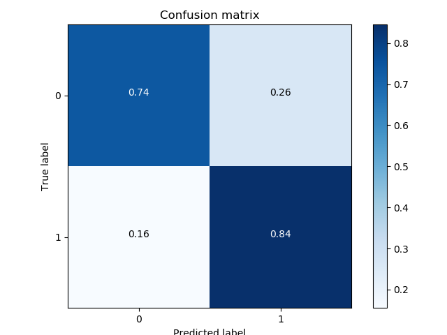
Precision Recall Curve
Precision Recall Curve shows the relationship between recall(x) and precision(y).
It is plotted by adjusting $thereshold$ when predicting labels. Given a trained classifier, we use it to predict some new samples, then we get a list of probabilities, if the probability is larger than $threshold$, we assign it as postive label, else we assign it as negative label. So when we adjust the threshold value, we will get a group of (precision, recall) pairs. Precision Recall Curve is plotted using these pairs.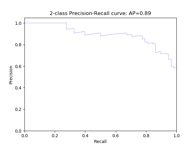
ROC curve and AUC of ROC
ROC Curve shows the relationship between TPR(x) and FPR(y).
$ TPR = \frac{TP}{TP + FN} $
$ FPR = \frac{FP}{FP + TN} $
Similar to Precision Recall Curve, ROC curve is also plotted by adjusting $thereshold$ when predicting labels.
AUC (area under curve) is the area under the ROC curve.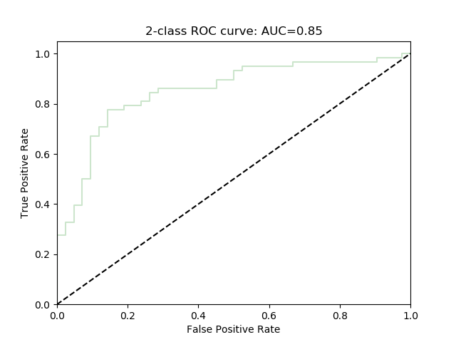
Trial
Finally, we use sklearn to train a binary classifier and evaluate this classifier using the above metrics.
|
|